I used 23,000 days of actual market data (dating back to the very end of 1927) in order to create my model. My goal was to explore the performance and profitability of Leveraged ETFs using the S&P 500 and Nasdaq-100 as benchmarks. I will both take an in-depth look into leveraged ETFs in this essay as well as explain my model.
To start, let me explain what a leveraged ETF is and why I thought this model necessary. Leveraged ETFs (Exchange Traded Funds) have the same structure as any other ETF and track different benchmark indices such as the S&P 500 Index, the Nasdaq Composite Index, Gold, Silver, and other commodity indexes. ETFs as a whole are a very popular way to diversify investments in safe, highly regulated, and liquid securities. Leveraged ETFs were originally invented to be used as a day traders’ tool to allow them to make more money off of small day to day price swings in the market than with traditional market tracking ETFs. The general principle for leveraged ETFs is that they multiply the gains and losses of the index they track by the amount they were meant too on a single day basis. This means that if the actual market rises 1% on a given day a leveraged ETF designed to move 2x the market would rise 2% on the same day. The same in reverse would happen if the actual market dropped 1% on a given day. Because leveraged ETFs are designed to follow the percent changes of the market on a day to day basis rather than for longer periods of time, this means that the leveraged ETFs could severely over-perform or under-perform the market over longer periods of time depending on market conditions that I will attempt to explain later.
Leveraged ETFs use financial derivatives contracts such as Swaps and sometimes futures which allow them to multiply the movements of the market. LETFs will also hold the individual stocks that make up the underlying index. The swap contracts constitute the majority of the LETFs notional value and are held between the LETF and large investment banks looking to hedge their investments. Generally, though not always, the long side of the swap contract (the side that is taken by the normal LETF) pays a certain percentage amount upon the notional value of the swaps usually based upon the current LIBOR rate plus some basis points to the short side (seller) of the contract which is detrimental to the performance of the LETF, especially in times of high-interest rates. It is also important to note that swaps are over-the-counter securities meaning they are highly individualized and customizable between parties. LETFs also use exchange-traded index futures contracts to a lesser degree (with the exception of commodity-based LETFs which usually only use futures). The most notable thing about the use of index futures is that they are generally in a state of backwardation which is beneficial to the performance of the index LETF. Finally, the leveraged ETF will hold the stocks that make up the underlying index in a small quantity compared to its notional value. The stocks pay dividends that are distributed to the shareholder of the LETF. The positions of the LETF are rebalanced at the end of every day. Some critics believe when a large-sized LETF sells stock shares to rebalance the portfolio in order to pay the swap counter-party after a negative market day, the downward pressure the selling of the shares would create would paradoxically force the market to move even lower the next day. This would create a constant negative feedback loop detrimental to the value of the LETF. I have not, however, seen any proof to this theoretical phenomenon actually happening since it is reasonable to believe that the quantity of the shares being sold during the rebalancing would usually have a negligible effect upon the market. There are also fees for ETFs known as expense ratios which are how the managers of the ETFs profit. These are always substantially higher on leveraged ETFs, often approaching 1% or more of the total assets.
There are also inverse ETFs that move in the opposite direction as the market such as SDS (-2x) and SPXU (-3x) which also use Swaps to function by taking the short side of the swap (though they often have to pay for the swaps even though the short side usually receives the swap rate). Because the stock market historically always rises when given enough time, short leveraged inverse ETFs are extremely bad long-term investments and only useful for short term speculation. Most of these inverse LETFs have lost 99%+ of their value since their inception. As they are very poor medium to long term (and even highly risky for the short term) investments I do not focus on them and will be referring to the inverse ETFs no more for the remainder of the article.
The market’s main influences upon leveraged ETFs as to their long-term success is market volatility. As I will try to show, market periods of high volatility (such as now) hurt leveraged ETFs a great deal while periods of low volatility allow leveraged ETFs to greatly outperform the market as long as the market is going at least very slightly upwards and minimize losses when the market is slowing declining or staying the same. The volatility of the market hurts leveraged ETFs even if the stock market is neither going up nor down during a period of time. The reason for this is because of the mathematics behind the percentage movements of leveraged ETFs. I shall illustrate this here:
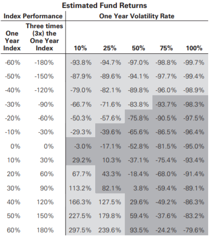
Taken from UPRO’s prospectus.
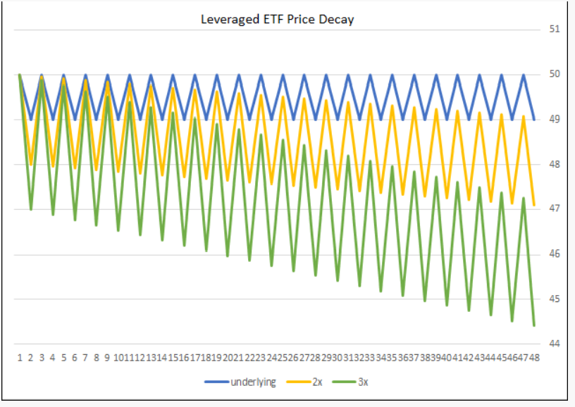
As you can see the price decays even when the underlying value of the market moves between the same two points the leveraged version decays in value. The mathematical reasoning behind this is that if you subtract 1% from 100 you have 99 and then if you add 1% of 99 to 99 you get 99.99 or almost exactly what you started with. However, if you subtract 3% from 100 you will get 97 and if you add back 3% to 97 you will get 99.91 which is not as close to the original number as the last example was. This effect will be even more devastating over a long period of time as shown by the table which was published in the prospectus of one of the leveraged ETF called UPRO. Also, the greater the leverage of the ETF the greater volatility hurts the ETF (2x is not as affected as 3x)
It is also important to note that leveraged ETFs perform extremely poorly in bear markets because they lose more than the market loses because of their leveraged nature. From my theoretical calculations (the actual leveraged ETFs didn’t start coming out until the mid-2000s), some of the higher multiple leveraged ETFs would lose as much as 95% and 99% of their value from during some of the worst financial crashes and depressions such as in 2001/2008 and the during the 1930s. With that said they recovered extremely quickly and grew to even higher levels than before. This investment strategy is not for those who are faint of heart or for those who aren’t willing to lock up their money for the foreseeable future. With that said over long periods of time, this investment strategy is unimaginably lucrative as my models will show. There are also certain ways to help the strategies become more stable and lucrative such as continually dollar cost average (as will be shown in my model). In times of low volatility, the leveraged ETFs are able to compound daily and therefore perform very well. This is why even though the leveraged ETFs are toted as a very short-term speculative tool (even the prospectuses of the ETFs say so), I believe that they can make a very lucrative long-term investment. Other things to note about leveraged ETFs is that they pay a much lower dividends rate than most S&P ETFs and have much higher expense ratios.
The last thing before I start explaining my model is that the actual leveraged ETFs have surprisingly outperformed what they theoretically should in my model, even with their expense ratios calculated in (which are very high for leveraged ETFs. UPRO (3x S&P) has an expense ratio of 0.92% while VOO (normal S&P) has an expense ratio of 0.03%). I have a portion of my model dedicated to this.
I downloaded my actual market data from Yahoo finance. The data has not yet been updated to take into account the market data from the months since the original creation of the model. The entirety of the model is essentially the equivalent of a rough and unpolished draft. There are several useless and random calculations and graphs as well as some repetition of calculations. I was learning as I built the model and tried several different ways to do things. Also, my naming conventions are not always constant. I always have graphs to the left of the data cells of each sheet for easy visualization. In some of my earlier graphs, the time axis is counting the rows of cells the data represents, or in other words the number of market days of data. Only later I found out how to change the actual counted number of days into time actual time periods and dates. I have not calculated the reinvestment of dividends into the performance of the baseline and the leverages. This doesn’t matter too much though as the dollar cost averaging would probably draw from the dividends instead of being on top of the reinvested dividends. I have also not yet included the theoretical expense ratio or swap costs yet; however, this point is lessened due to the fact that the actual leveraged ETFs have historically (during there so far short lifetimes) beat what they theoretically should have performed even when expense ratio and the costs of swaps are included in the actual performance and not in the theoretical. It is also hard to guess what the expense ratios would have been in the past as all ETFs and Mutual Funds have gone down in Expense Ratio greatly over the years (and Index tracking Funds are a considerably newer invention without even mentioning the newness of the leveraged ETFs). My volatility versus the performance section is not yet complete as I struggle to find a way to quantify the correlation. Volatility is greatly based on statistics which is a subject I am not yet very well versed with. Finally, I need more starting points and time ranges in order to solidify the usefulness in my results and I may add a way to change the volatility and actual growth of the S&P to play around with different factors without relying on actual market data (to make it a true model).
Here is the spreadsheet download.
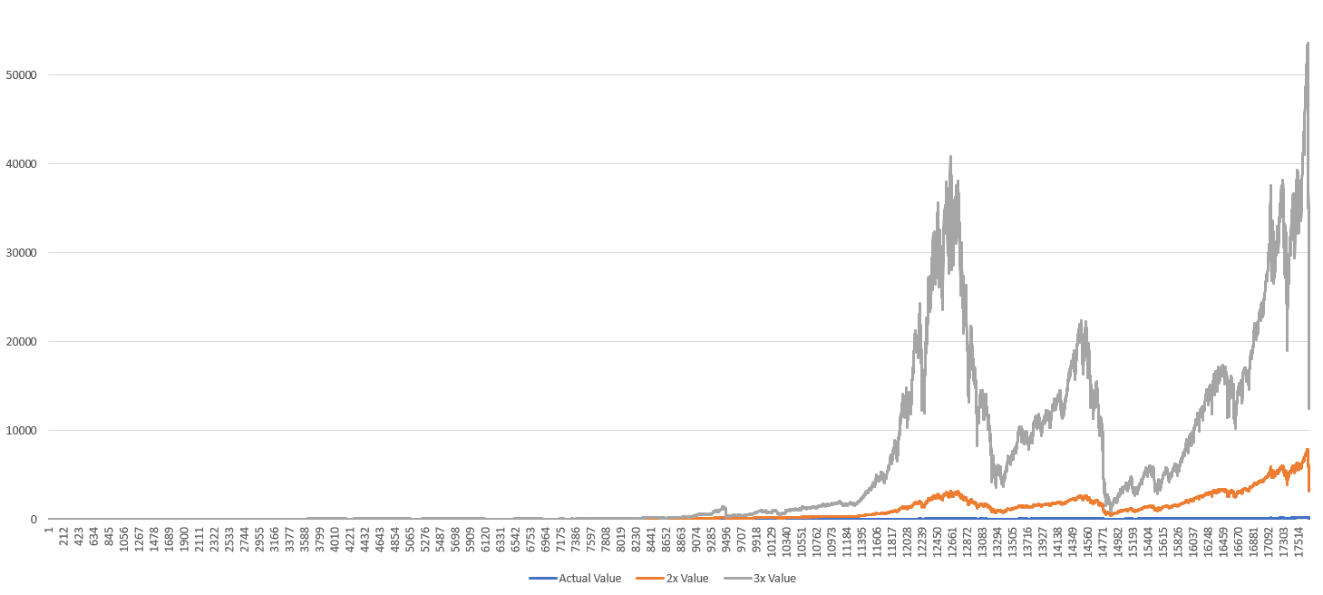
The first sheet in the model contains 23,000 days of data and compares the different leveraged ETF’s theoretical performance in comparison to the actual market performance of the S&P 500. The value of each test is in terms of the S&P value so that each test starts at a beginning value of 17.66 because that’s the number the S&P index valuation is equal to at the beginning date of the test. The results of this test surprised me as I originally believed that the 3x would perform better than the other variations; However, the 2x greatly outperformed the 3x. I was even more surprised to dee that the 1.5x also performed very well compared to the 3x. The 3x performed worse than the actual S&P for most of the length of time. I believe this is due to the test starting right before the great depression and this really hurt the 3x. I tried various other leverage amounts but none of them performed as well as the 2x. It was proposed to the SEC to have a 4x leveraged ETF but the SEC denied its creation because they believe it would be too risky for the common investor. I threw the 4x into the model anyways and as it turned out while it had its moments of success it would mainly have performed terribly of the course of the past 90 years. Even though I didn’t keep them in the model, I tried variations close to 2x such as 1.75x, 2.25x, and 2.5x to see what was really the most efficient leverage amount. I found that 2x was, in this scenario, really the best leverage amount. On top of that, the real leveraged ETFs don’t have any of those latter leverage multiples currently available of products, so it doesn’t really matter anyway. The results were that the 2x would have peaked about a month ago at a value of almost 25,000 versus the actual S&P 500 that peaked at about 3,400.
I then moved on to checking my theoretical results with the leveraged ETF’s actual results. I only checked against two of the different multiples of the leverages as those were the ones, I was most interested in: 2x and 3x. The actual 3x I used to test my theoretical against is an ETF with a ticker symbol of UPRO. It has been around since 2009 so that’s when the test starts. UPRO does about 10% (and because it is exponential growth it would continue to widen the performance gap if there was a longer period of data) better than what I calculated it theoretically does even with expense ratio calculated into its performance. I still am not completely sure why it performs so much better, but when put into perspective, the % of higher gain the theoretical would need to match UPRO’s actual record is about +0.013% each day above the actual 3x price change of the market. This could easily be due to a small rounding error or transactional difference and only is noticeable after long periods of time. I also tested the theoretical 2x against its real-life equivalent that has the ticker SSO. Once again, the actual beat the theoretical but this time by a slightly smaller margin (even though SSO has a lower expense ratio than UPRO). SSO IPO’d in 2006 so that’s when the test starts for the 2x. It’s important to note that since the real leveraged ETFs haven’t been around for much longer than a decade this enhanced performance may not continue into the future, and may in fact in a worst-case scenario reverse itself.
Because I thought the lackluster results of the 3x were strange, and because I believe starting the trial right before the greatest economic crisis of at least recent history may have skewed the results, I did a trial with a starting date in 1950. In this case, the 3x did way outperform the 2x and all other multiples. I also threw in 4x to the test and found that 4x would have performed extremely well around the late 90s but then crash down to mostly perform worse than 3x thereafter. It may theoretically perform extremely well again in the future, but I am going to have to look at factors that make it perform so well. In this sheet, I also adjusted the starting value to 1 in order to more easily see their growth over the time period. This means that at its peak a theoretical investment in a 3x leveraged ETF would have returned an amount over 50,000 times the original investment at its recent peak in early 2020 over the course of about 70 years while investing in the regular S&P would have created an increase of about 200 times its original investment at its recent peak.
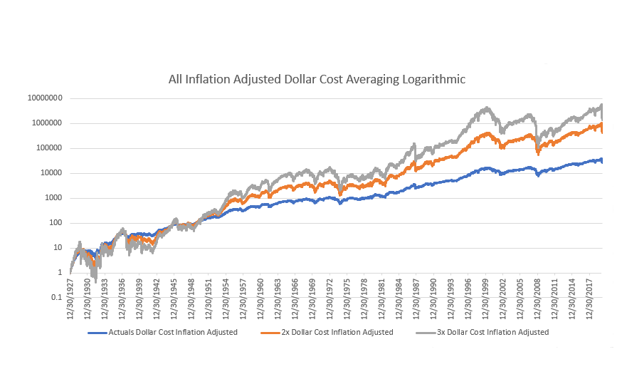
I wanted to find a way to make the 3x give more consistent results as the winner so I added dollar-cost averaging and continual investment in the equation and the results were satisfactory. Before going back to 1929 as a starting point I tried testing it from the 1950 starting point. The principal behind the dollar cost averaging is that a person puts in their initial investment and then adds an additional 1% of the original investment to it every day thereafter. As in you would enter an amount of $100 to start out with and then add another $1 into the investment every day thereafter. The idea behind this is that the investor would buy at all points of the market cycle, including the low points, and therefore make more money on the way up. Also, realistically a person is continually making more money from their main source of income is naturally going to invest some of it. 1% may seem like a high amount to have to invest every day (an investor may have a large sum of money saved up to put initially into this investment through their actual income wouldn’t allow them to invest such a high percentage of the original more each day), and the model allows for an easy change in dollar-cost percentage and can be changed to match possibly more realistic quantities such as .1% per day or .01%. Though the outcomes are not as good as investing 1% more per day they still do very considerably better than just one lump sum upfront. This does not mean however that an investor should break up their initial investment and invest it slowly into the market, as investing the most possible upfront usually does result in much higher returns unless the starting point is right before an economic depression. The idea is rather simply to invest even greater amounts as the cash comes available through dividends or other sources of income. Also, there is no need to invest on a daily basis because realistically on a monthly would do just almost as well and makes more sense for most people. The reason that in the model it is 1% more on a daily basis rather than about 30% on a monthly basis as it was easier to calculate into the model and it would also probably perform slightly better than reinvesting on a monthly basis due to compounding effects. The outcome of investing 1% more of the original investment on a daily basis is that the returns for the 3x are almost 450,000 times the original investment at its 2020 peak over the course of about 70 years.
I then tried the dollar-cost averaging for the period starting in 1929 and found that the 3x did in fact beat everything else by a very large margin. An original $1 investment would have turned into about $3.5 million over the 90-year period when $0.01 was added to it every day. If you remember the non-dollar cost averaging 1929 starting point had a 3x lag in performance. Through my calculation, if you had added on average as little as one basis point (0.01%) of the original investment to the investment every day the ending results would have the 3x outperforming all the other variations by the current date (though not by as high as an amount as if the dollar cost average amount had been greater than 0.01%). I also realized how inflation would make the additional 1% daily additional investment an extremely small amount by the end of the test period so I added an inflation adjustment to the dollar-cost averaging. I figured the average inflation rate from the 1930s to the present was about 3% a year on average so I increased each day’s dollar-cost percentage by that amount divided by the number of trading days in each year. It by no means is a perfect inflation adjustment and does not actively change in growth during times of greater than normal inflation or decrease in times of deflation though it does give a pretty good average inflationary amount and can also take into account things such as work promotions and the pay raises that come with them (as people on average make more and more money as they become older and more experienced). In current times the daily dollar-cost averaging is about 15 times the original starting point in 1929. As it turns out that the theoretical performance of dollar-cost averaging does not increase all that much due to the inflationary adjustment as the smaller quantities of money invested earlier very much outweigh the later larger quantities of investment in value. However, I do believe it is important because the longer you keep up this investment the more adjusting for inflation becomes important and it is also a more realistic way to make the model. Also, it allows for much faster recoveries after times of turmoil such as in 2008 as you are investing more money into the leveraged ETFs than ever before exactly when it is best to invest more than usual.
My next sheet is still a work in progress but the idea for it is to be able to measure how much volatility actually effects the performance of these securities. I am still thinking of ways to best represent this. I am using volatility measures such as the VIX (Volatility Index) in order to perform this task. VIX dates back to 1990 so that is the starting point of this experiment. As I stated before my this is very statistically-based and therefore not my strong point.
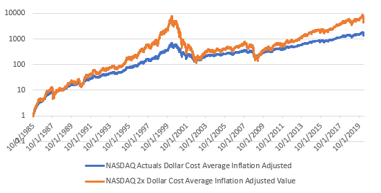
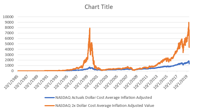
I also repeated the tests I performed in with the S & P but with the NASDAQ-100 starting in 1985 (when the index was introduced). There are two pages dedicated to this which cover the theoretical performance and the performance versus reality. The results are such that the theoretical tracked the actual very closely. The theoretical 3x gained a near 800,000% at its peak in 2020 giving it an annualized return of approximately 38%. The spike during the dot-com boom is also noteworthy.
I have been shaping my investment strategy off of this model. As it is always unknown how the markets will actually perform in the future this investment strategy is only for those who are able to tie up money for long indefinite periods of time and have large risk tolerance (mostly younger people) though I am certain that this strategy will prove to be extremely lucrative to me (I can only guess as to whether or not it will be as lucrative as it would have theoretically been in the past). As for my picks of leveraged ETFs, I choose UPRO, the 3x S&P 500 tracking ETF and TQQQ, the 3x NASDAQ-100 tracking ETF. Even though TQQQ has beaten UPRO historically instead of investing all in TQQQ I still want to diversify into both because the NASDAQ has not been around nearly as long as the S&P and therefore it is unknown as too whether it will continue its outstanding performance in the future.
Additional resources:
Dynamics of Leveraged and Inverse ETFs Powerpoint